Portfolio Visualizer with Matplotlib in Python

Introduction

Python is the number one language for machine learning and data science right now. For the most part this is because of the powerful external libraries, that allow us to train machine learning models and visualize data with just a few lines of code. In this tutorial, we are going to use Matplotlib, in order to visualize a stock portfolio. Our end result will look like the chart below.

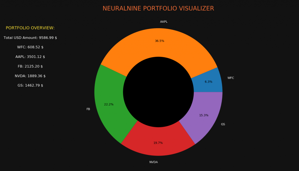
As you can see, we will visualize the distribution of the invested money while also giving information about the actual dollar amount invested in the various companies.

Perquisites

For this tutorial, we will need to install and import some libraries. To do this, you can use a tool like pip. The external libraries that we are going to use are Matplotlib and Pandas-Datareader. The first one will be used for all the visualization and the second one will be used for loading the stock data. Notice that for the Pandas-Datareader you will also need to install Pandas itself. Also, we are going to import the Datetime module from Core-Python.

import datetime as dt
import matplotlib.pyplot as plt
from pandas_datareader import data as web

Other than that you will just need some basic understanding of the Python language. You need to understand lists, loops, data types and so on. Being familiar with the stock market might also be beneficial.

Loading Data

The first step of our script will be to set up our portfolio and load the stock data from the Yahoo Finance API. For this, we will create a couple of lists with our stocks and then use the Pandas-Datareader to load the respective data.

tickers = ['WFC', 'AAPL', 'FB', 'NVDA', 'GS']
amounts = [12, 16, 12, 11, 7]
prices = []
total = []

We create four lists. The first one has all the ticker symbols of the companies that we have in our portfolio. In the second list we find the amount of shares owned of these stocks. The prices list is empty and it will be filled with the share prices that we are going to load. And the last list will contain the calculated total positions for each company. If you want, you can also modify your script so that the user can input these values when running the script.

If you need more information about the stocks themselves or their ticker symbols, check out the Yahoo Finance API.

for ticker in tickers:
    df = web.DataReader(ticker, 'yahoo', dt.datetime(2019,8,1), dt.datetime.now())
    price = df[-1:]['Close'][0]
    prices.append(price)
    index = prices.index(price)
    total.append(price * amounts[index])

Now we run a for loop that iterates over our tickers. For every ticker symbol, we download a data frame from the Yahoo Finance API. Notice that I just picked a short timeframe here. It is important that you choose now as an end date. The starting date is not that important but it should be relatively recent.

When we have loaded the data frame into our script, we slice it and pick the last closing value. This value then gets appended onto our prices list. Finally, we calculate the total position by multiplying the amount of shares by the share price. We now have four filled lists and the rest is just visualization.

Visualizing The Portfolio

The visualization is actually very simple since there is almost no logic involved. However, we will use a lot of different functions and parameters for our design, which might be confusing. Keep in mind that once you know the functions, everything is very simple.

fig, ax = plt.subplots(figsize=(16,8))

ax.set_facecolor('black')
ax.figure.set_facecolor('#121212')
ax.tick_params(axis='x', colors='white')
ax.tick_params(axis='y', colors='white')

ax.set_title("NEURALNINE PORTFOLIO VISUALIZER", color='#EF6C35', fontsize=20)

In the first line we just create our figure and our subplot. The parameter here only defines the size of the figure. After that, we set the color of the actual plot to black and the color of the figure to a very dark gray. Because of that, we want our tick-parameters to be white. We also add a title with the orange color of NeuralNine. Of course you can change this.

patches, texts, autotexts = ax.pie(total, labels=tickers, autopct='%1.1f%%', pctdistance=0.8)
[text.set_color('white') for text in texts]

my_circle = plt.Circle((0, 0), 0.55, color='black')
plt.gca().add_artist(my_circle)

Now we get into the essential plot. Since Matplotlib doesn’t offer any functions for plotting a donut chart or a ring chart, we will need to get creative. What we do is, we plot an ordinary pie chart and put a black circle in the middle of it. So first we use the pie function to flot the total values with the respective tickers. Also, we add the percentages which we then position at a higher distance from the center, because we need to make space for our black circle.

Notice that we have three variables that get values returned by the pie function. We are interested in the text variable because we want to change the color of the tickers. For this, we use an inline for loop to set the color of all texts to white.

After all that we create a new Circle object and place it into the middle of the screen which is (0,0). We give it a radius of 0.55 and a color of black. To now add the circle to our plot, we need to use the gca function which stands for get current axis and add it with the add_artist method.

ax.text(-2,1, 'PORTFOLIO OVERVIEW:', fontsize=14, color="#ffe536", horizontalalignment='center', verticalalignment='center')
ax.text(-2,0.85, f'Total USD Amount: {sum(total):.2f} $', fontsize=12, color="white", horizontalalignment='center', verticalalignment='center')
counter = 0.15
for ticker in tickers:
    ax.text(-2, 0.85 - counter, f'{ticker}: {total[tickers.index(ticker)]:.2f} $', fontsize=12, color="white",
            horizontalalignment='center', verticalalignment='center')
    counter += 0.15

plt.show()

Our visualization is pretty much done but we also want to add some text with the stock data to it. For this we use the text method. We adjust parameters like the font size, the color and the alignment. Notice that from the second line on we are using string formatting to display our values.

Now for plotting the texts of the individual values I got a bit creative. I created a counter variable which is used for positioning our texts. To display the individual stock positions, we iterate over the tickers and plot the text. However, we need to change the y-coordinate and because of that, we always subtract 0.15. That might not be the most beautiful solution but it works. If you find a better one let me know in the comments!

As shown in the beginning, this is what our final result looks like. Feel free to make some changes to the colors, the stocks and the whole plot in general.

I really hope you enjoyed this tutorial! Feel free to ask questions in the comments! If you liked this post and are interested in more Python for Finance, Data Science and Machine Learning, you might want to check out my book series The Python Bible!

Also, check out the NeuralNine Instagram page for daily infographics, challenges and quotes!

PYTHON BIBLE 5 IN 1

FOR BEGINNERS

Follow NeuralNine on Instagram: Click Here

Subscribe NeuralNine on YouTube: Click Here

This Post Has 2 Comments

Tim 2. December 2019 Reply

Thanks, nice article. I thought the ‘yahoo’ API was decommissioned and the above way of extracting stock market data doesn’t seem to work for me. Have you tried it recently? I found documentation about a new library called “yfinance” to overcome the problem. I’d appreciate your thoughts.
1. Administrator 11. December 2019 Reply
  
  Are you sure? For me it still works perfectly fine. Sometimes it is buggy! But this script still works for me! 🙂