Linear Regression From Scratch in Python

Introduction

One of the most basic machine learning models is the Linear Regression. The purpose of linear regression is to take a bunch of data points and to draw a straight line right through them. This line should then be as near as possible to all the points. When we have found this line, we can use it to make predictions for future values. The following image shows a linear regression line.

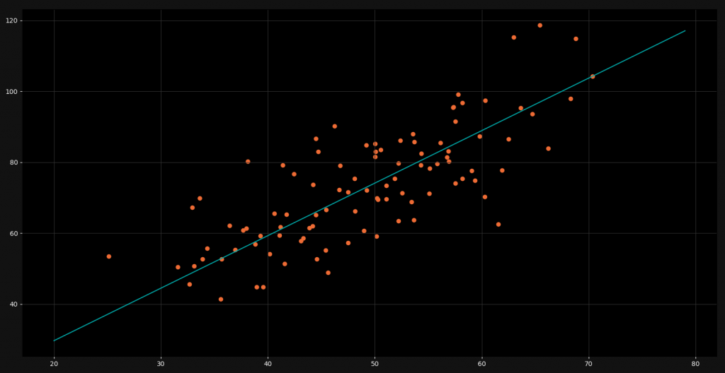
As you can see we have a lot of orange data points. For every x-value we have a corresponding y-value. The linear regression line is right in between all of these points and gives us a good approximated y-value for ever x-value. However, linear models usually unfold their potential only in higher dimensions. There they are very powerful and accurate.

But how do we find this optimal regression line? Of course we could just use a machine learning library like Scikit-Learn, but this won’t help us to understand the mathematics behind this model. Because of that, in this tutorial we are going to code a linear regression algorithm in Python from scratch.

Perquisites

Although we are programming this algorithm from scratch, we are going to use two data science libraries, namely Pandas and Matplotlib. Pandas will be used to import CSV-data into our script and Matplotlib will be used for the visualization of our model.

import pandas as pd
import matplotlib.pyplot as plt

Also it would be very beneficial for you to have a decent understanding of high school math and calculus. These are not inalienable for the programming but definitely for the understanding of the mathematics behind linear regression. You will need some basic knowledge about partial derivatives. But if you are just here for the code and you don’t care too much about the mathematics, you can go on as well.

Basics of Linear Regression

Now let us take a look at the basic structure of a linear regression. Since our model is a linear function it has the following structure:

$y = m * x + b$

Here m is the gradient and b is the intercept. Therefore we have two unknown parameters that we need to figure out. We can do this by using a loss function and the so-called gradient descent algorithm.

Loss Function - Mean Squared Error

Now in order to figure out these two values, we need to know how far away we are from the optimal line. In other words: We need to find out how far away our line is from each point. For this we use a loss function and in this particular case, we use the mean squared error loss function.

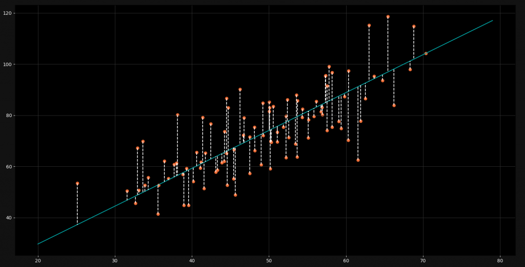
As you can see, every point has a certain distance to the regression line. This is the error or loss for that particular point. It indicates how much our model is off with the value. By using the mean squared error loss function, we now take all these errors, square them, add them up and then divide by the amount of points. In other words: We take the mean of the squared errors for all the points.

$E = \frac{1}{n} \cdot \sum_{i=0}^n (y_i – \overline{y_i})^2$

This is the mathematical way of writing down what I’ve just explained. For every element, we calculate the difference between the actual y-value and the y-value of our regression line and we square it. Then we multiply the sum of all these squared errors by 1/n which is the same as dividing it by n. Then we get our mean squared error. If we insert the formula for the y-value of the regression line, it looks like this:

$E = \frac{1}{n} \cdot \sum_{i=0}^n (y_i – (m \cdot x_i + b))^2$

Now we have a great loss function to determine how far we are away from the perfect regression line. Our goal is now to minimize the value of this loss by changing the m and the b parameters.

Gradient Descent

For minimizing the output of the error function, we will use an optimization algorithm known as gradient descent. What it basically does is trying to find the local minimum of a function, by looking at the steepness of a slope in a specific point and taking steps towards the “valley” of the function. The steeper the slope, the larger the steps.

So what we need to do is to find out how the output of our loss function changes, when we change our two parameters (m and b). For this, we will need to compute the partial derivatives. This is the part where you should be familiar with calculus to understand exactly why things are the way they are. If you are just interested in the code however, you can just keep reading without understanding every detail.

We start by letting the values of our two parameters be zero (let m = 0 and b = 0). Additionally, we need to define a so-called learning rate. This controls how much we want to change the individual values with each step. The smaller L is, the more accurate our model will be. If it is too small however, it will take a very long time to be trained. A learning rate of 0.0001 is a good choice.

$\frac{\partial y}{\partial m} = \frac{1}{n} \cdot \sum_{i=0}^n 2(y-(m \cdot x_i + b))\cdot(-x_i)$

When we now restructure this equation a little bit, it looks like this:

$\frac{\partial y}{\partial m} = -\frac{2}{n} \cdot \sum_{i=0}^n x_i\cdot (y-(m \cdot x_i + b))$

Now what we have here is the partial derivative of the mean squared error loss function for m. This function tells us how the output of the loss function changes when when we make a slight change in m. But to optimize the whole function, we need to do the same thing for b.

$\frac{\partial y}{\partial b} = -\frac{2}{n} \cdot \sum_{i=0}^n (y-(m \cdot x_i + b))$

These two functions give us the information how much we need to change our parameters. Last but not least, we need to apply the changes in every iteration.

$m = m – L \cdot \frac{\partial y}{\partial m}$

$b = b – L \cdot \frac{\partial y}{\partial b}$

As you can see, the learning rate is important because it defines how much we apply the change of our parameters. So, enough of the math behind linear regression. Let’s get into the code!

Implementing Linear Regression in Python

As I already mentioned in the beginning we will need the two libraries Matplotlib and Pandas for loading and visualizing the data.

import pandas as pd
import matplotlib.pyplot as plt

The next step is to load our data from a CSV-file into our script. For this tutorial we are using a simple file with some x-values and y-values. You can download it here! Alternatively, you can also use your own custom CSV-file.

points = pd.read_csv('data.csv')

Now that we have our data in the script, we can start defining our functions. Let’s start with the loss function.

def loss_function(m, b, points):
    total_error = 0
    for i in range(len(points)):
        x = points.iloc[i, 0]
        y = points.iloc[i, 1]
        total_error += (y - (m * x + b)) ** 2
    return total_error / float(len(points))

Basically, we are just putting the mathematical equation into code. We have three parameters – m, b and points. The points are the data points from our CSV-file. We iterate over all the individual points and calculate the squared error for each of them. To access the points, we use the iloc functon, which allows us to select elements from the data frame. At the end, we just divide our summed squared errors by the amount of points to get the mean. Next we need to define the gradient descent function.

def gradient_descent(m_now, b_now, points, L):
    m_gradient = 0
    b_gradient = 0
    n = float(len(points))
    for i in range(len(points)):
        x = points.iloc[i, 0]
        y = points.iloc[i, 1]
        m_gradient += -(2/n) * x * (y - (m_now * x + b_now))
        b_gradient += -(2/n) * (y - (m_now * x + b_now))
    m = m_now - L * m_gradient
    b = b_now - L * b_gradient
    return [m, b]

Once again, we just implement the mathematics from before. We iterate over each points to calculate the partial derivative for m and b. In that way we know how steep the slope is at these points. At the end we return the new calculated values for m and b. The learning rate decides how strong we change these values.

Now actually training the model is very easy. We just need to define some initial values and then apply our funcitons.

m = 0
b = 0
L = 0.0001
epochs = 1000

for i in range(epochs):
    m, b = gradient_descent(m, b, points, L)

print(m, b)

First we set our two parameters to zero as explained before. Then we define our learning rate to be 0.0001 which is quite a good value for this task. The last important value is the amount of epochs. It defines how many times we are going to apply the gradient descent algorithm over and over again. We then just run our loop and optimize our values. Finally, we can print our results.

1.4607911678007937 0.08980028357345672

Visualizing and Animating

For the mathematical machine learning part we are done, but in order to understand the principle fully, we will use Matplotlib to animate and visualize the linear regression. We will first need to restructure our code a little bit. First of all, we are going to set our epochs to 100 and our learning rate to 0.00001 in order to see better what is happening while training our model.

L = 0.00001
epochs = 100

Now to animate the training process with Matplotlib, we will need to turn on the so-called interactive mode by using the ion function. We are also going to define two subplots in our figure. The first one will visualize our data points and our regression line, whereas the second will plot the development of the loss function output.

plt.ion()

fig = plt.figure()
ax1 = fig.add_subplot(211)
ax2 = fig.add_subplot(212)

ax2.set_xlim([0,epochs])
ax2.set_ylim([0,loss_function(m,b,points)])

ax1.scatter(points.iloc[:,0], points.iloc[:,1])
line, = ax1.plot(range(20, 80), range(20, 80), color='red')
line2, = ax2.plot(0,0)

We are setting the limits of the second plot to the amount of epochs on the x-axis and to the initial loss function output (since it will only decrease from here) on the y-axis. Then we scatter all of our points onto our first plot. After that we define the initial values for our two animated functions. For our regression line we start with the initial values from 20 to 80 since all of our points are within that range. Notice that the x-values will stay constant here and only the y-values will change. For our second line we define zero and zero. Here we will change both values. The x-value will increase with every epoch and the y-value will show the loss function output.

xlist = []
ylist = []

for i in range(epochs):
    m, b = gradient_descent(m, b, points, L)
    line.set_ydata(m * range(20, 80) + b)

    xlist.append(i)
    ylist.append(loss_function(m, b, points))
    line2.set_xdata(xlist)
    line2.set_ydata(ylist)

    fig.canvas.draw()

plt.ioff()
plt.show()

Finally, we are getting into the actual plotting. We define two empty lists, which we will fill with the data necessary for our loss function plot. Notice that we have now placed the loop with the training function here and combine it with the animation. With every training iteration we update our graphs by using the functions set_xdata and set_ydata. To make the changes visible, we update our plot in every iteration by using the draw function of the canvas. At the end, we turn off the interactive mode and show our final plot.

Styling and Design

When you execute your script, you will see that the design doesn’t look like a NeuralNine design. For this reason, we are going to change the style a little bit. This has to be done before showing the plots.

fig.set_facecolor('#121212')
ax1.set_title('Linear Regression', color='white')
ax2.set_title('Loss Function', color='white')
ax1.grid(True, color='#323232')
ax2.grid(True, color='#323232')
ax1.set_facecolor('black')
ax2.set_facecolor('black')
ax1.tick_params(axis='x', colors='white')
ax1.tick_params(axis='y', colors='white')
ax2.tick_params(axis='x', colors='white')
ax2.tick_params(axis='y', colors='white')
plt.tight_layout()

We are basically changing the color scheme to be dark gray and black. Also, we are setting titles for our plots and using the tight_layout function, so make everything well aligned. Now we can also change the colors for our points and functions.

ax1.scatter(points.iloc[:,0], points.iloc[:,1], color='#EF6C35')
line, = ax1.plot(range(20, 80), range(20, 80), color='#00ABAB')
line2, = ax2.plot(0,0, color='#00ABAB')

Now our plot finally looks like this:

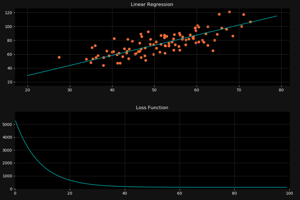
I hope you enjoyed this blog post! If you want to tell me something or ask questions, feel free to ask in the comments! Check out my instagram page or the other parts of this website, if you are interested in more! Stay tuned!