Handwritten Digits Recognition With Tensorflow

Introduction

One of the most powerful and most popular libraries for machine learning out there is Tensorflow. It allows us to easily build, train and use neural networks. In this tutorial, we are going to use Tensorflow, in order to recognize handwritten digits by training a deep neural network. However, we are not going to get into the mathematics of neural networks (this will be a topic of the future), nor will we talk about the optimizers or loss functions in too much detail. Here we will focus on the use case and just implement the functionality. We will build and train a neural network that will be able to classify our own handwritten digits with a very high accuracy.

Perquisites

For this tutorial, we will need to import a couple of libraries. If you are only interested in the training and testing of the model, you will only have to import Tensorflow. However, if you also want to read in your own handwritings, you will need to import a couple more libraries. Almost all of these libraries are external and need to be installed with some tool like pip.

import os
import cv2
import numpy as np
import tensorflow as tf
import matplotlib.pyplot as plt

We will use Tensorflow for all of the machine learning. The other libraries will help us to scan our own images into the script. Cv2 will read the images, which will then be restructured with NumPy and displayed with Matplotlib. Also, we will use os to check if certain files exist.

Loading The Data

Now the first thing we need to do is obviously to get some training data first. For our neural network to be able to predict handwritten digits, it first needs to be trained on many thousands of images. Therefore, we are going to use the so-called MNIST data set of handwritten digits. It has a training set of 60,000 images and a test set of 10,000 images. These images have a resolution of 28×28 pixels. We can directly import it from Tensorflow.

mnist = tf.keras.datasets.mnist
(X_train, y_train), (X_test, y_test) = mnist.load_data()

When we call the load_data function here, we get two tuples as an output. The first one contains the training values for x and y and the second one the test values for x and y. Our x-values are the features (in this case the 784 input pixels) and our y-values are the respective digits. The next step is to now normalize our data.

X_train = tf.keras.utils.normalize(X_train, axis=1)
X_test = tf.keras.utils.normalize(X_test, axis=1)

By normalizing our data we divide each data point by a constant. This means that the data still has the same patterns and gives us the same information but it also makes computation easier. Notice that we are only normalizing the x-values, since the y-values need to stay the way they are (digits from 0 to 9).

Building The Neural Network

After loading and normalizing our data, we can now start to build our neural network. For this we use Tensorflow and simply define our model and the individual layers.

model = tf.keras.models.Sequential()
model.add(tf.keras.layers.Flatten(input_shape=(28,28)))
model.add(tf.keras.layers.Dense(units=128, activation=tf.nn.relu))
model.add(tf.keras.layers.Dense(units=128, activation=tf.nn.relu))
model.add(tf.keras.layers.Dense(units=10, activation=tf.nn.softmax))

Now this might be confusing when you look at it for the first time. But actually it is quite simple. The first thing that we are doing here is to define our basic neural network model. We create a Sequential model. This is a linear type of neural network, which is defined layer by layer. It is the default type you use for this kind of task.

After that, we always use the add function to add new layers to the model. So every line defines a new layer. We start out with a Flatten layer for our inputs. This type of layer flattens the input. As you can see, we have specified the input shape of 28×28 (because of the pixels). What Flatten does is to transform this shape into one dimension which would here be 784×1.

Following the input layer, we add two Dense layers which are our hidden layers. These make our model more abstract and sophisticated. Dense is the default layer type and it just means that every neuron is connected to every other neuron of the neighboring layers. In this case, we choose two layers with 128 neurons each. You might ask yourself what the optimal amount of layers and neurons is. It totally depends on your ressources. But if you want a detailed table, check out this link. What you will also notice is that we are specifying an activation function. This function determines when and how intense a neuron will fire. Here we chose the RELU function, which stands for Rectified Linear Unit.

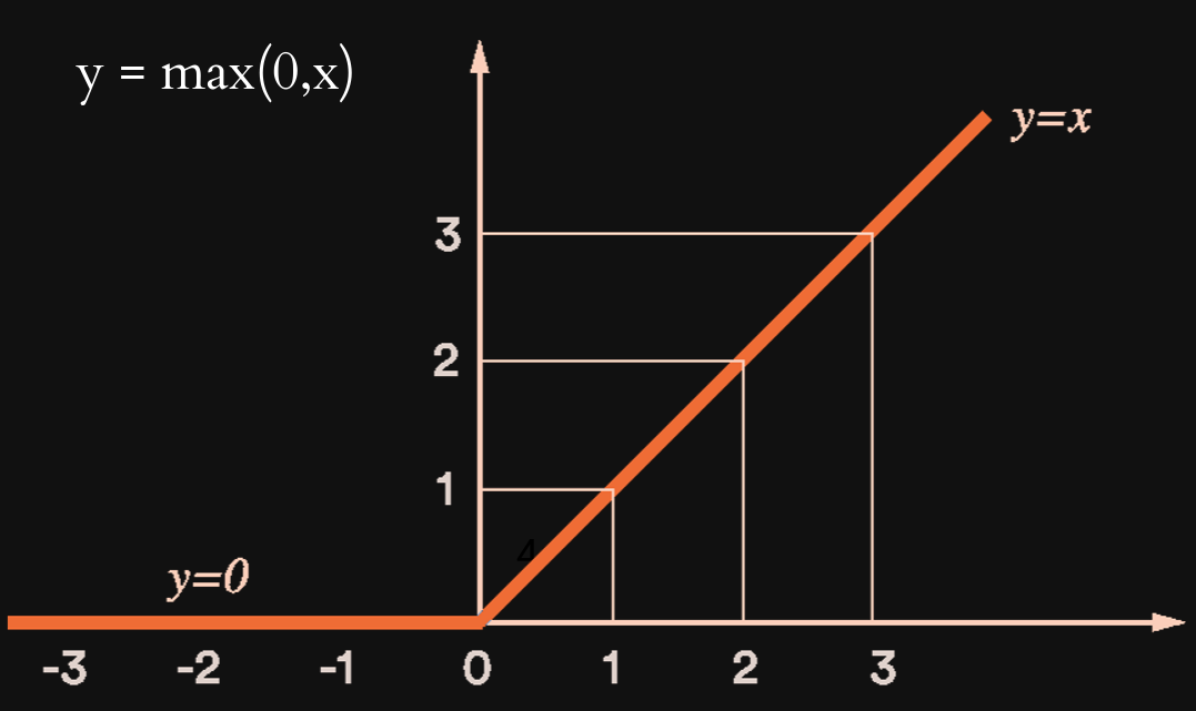
It is very simple. When all the inputs of a neuron are summing up to a negative number, the neuron doesn’t fire and the output is zero. In every other case however, the neuron outputs its input. Although this function is extremely simple it is quite powerful and oftentimes used.

So last but not least, let us get to the last layer. This is the output layer and it also is a Dense layer. But this time we only have ten neurons (because of the ten possible digits) and a different activation function, namely Softmax. Softmax takes all the outputs and makes them add up to one. In other words: For each digit we will get a number that indicates how likely this digit is the correct result. All the probabilities will then obviously add up to one.

Now our model is build and we just need to compile it. By doing this we define certain parameters and configure it for training and testing.

model.compile(optimizer='adam', loss='sparse_categorical_crossentropy', metrics=['accuracy'])

Here we define three things, namely the optimizer, the loss function and the metrics that we are interested in. As I already said, we will not go into too much detail or mathematics here. Therefore, we are not going to explain the Adam optimizer or the loss function we use. However, these are very popular choices, especially for tasks like these.

Training And Testing

Our model is now built and we can start training and testing it. With Tensorflow training our model is made very easy, since it only needs one line of code.

model.fit(X_train, y_train, epochs=3)

Here we need to pass three parameters. The x-values, the y-values and the number of epochs. By passing the training data, our model recognizes the relationships between the pixels (x-values) and the digits (y-values). After 60,000 examples, it should be quite good at recognizing digits. The epochs define how many times we are going to feed the same data into our model. Everytime we feed data into our model, it adjusts its parameters. By feeding in the same data multiple times, it gets more and more accurate. However, if we carry that too far, we might overfit the model. This would lead to a model that is very good at classifying the digits it already knows but performs terrible on new and unknown data.

After our model is trained, we can now evaluate or test it. For this, we are intrested in two values – the loss and the accuracy.

loss, accuracy = model.evaluate(X_test, y_test)
print(loss)
print(accuracy)

Predicting Custom Digits

Now the last part is to load our own images into our script. For this you may either scan real handwritten digits into your computer and scale them down to 28×28 pixels or you can use paint to draw 28×28 pixel digits. I will do the latter.

In this case, we will create around ten drawings and save them into a directory. To make it easier for us, we will create a digits folder with all images in it. The file names will have the structure digit_.png.

image_number = 1
while os.path.isfile('digits/digit{}.png'.format(image_number)):
    try:
        img = cv2.imread('digits/digit{}.png'.format(image_number))[:,:,0]
        img = np.invert(np.array([img]))
        prediction = model.predict(img)
        print("The number is probably a {}".format(np.argmax(prediction)))
        plt.imshow(img[0], cmap=plt.cm.binary)
        plt.show()
    except:
        print("Error reading image! Proceeding to the next one...")
    finally:
        image_number += 1

Above you can see the whole code for our loading, predicting and visualizing. The first step is to run a while loop for as long as there are new digits to load in our folder. Then for each file we use the imread method to load it. However, we need to drop one dimension here so that we have the right shape. In order to not confuse our model, we also need to invert our image so that it is black on white.

After that we use our model to predict the class for our image array. Since we used the softmax activation function for our output layer, we need to use the argmax function on our prediction, to get the class with the highest probability.

Last but not least, we use the imshow function to display our digit and with every iteration, we increase the image number by one. That’s it! Our model is done and we can predict our own handwritten digits with an accuracy of around 97 percent.

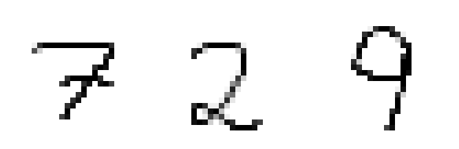
The number is probably a 7
The number is probably a 2
The number is probably a 9

As you can see, it works very well! I really hope you enjoyed this tutorial! Feel free to ask questions in the comments! If you liked this post and are interested in more Python and Machine Learning, you might want to check out my book series The Python Bible!

Also, check out the NeuralNine Instagram page for daily infographics, challenges and quotes!

PYTHON BIBLE 5 IN 1

FOR BEGINNERS

Follow NeuralNine on Instagram: Click Here

Subscribe NeuralNine on YouTube: Click Here